XGBoost: The Magic Behind Our Fusion Model

What Is XGBoost?

XGBoost stands for eXtreme Gradient Boosting. It's one of the most powerful machine learning algorithms for structured data (like tables of numbers).

In competitions like Kaggle, XGBoost dominates because it's:

• Fast (parallel processing)

• Accurate (handles complex patterns)

• Robust (resists overfitting)

• Interpretable (tells you which features matter)

How Gradient Boosting Works

Boosting is an ensemble method: you combine many "weak learners" (simple models) to create one "strong learner."

Here's the intuition:

1. First tree – Make a simple prediction. It will be wrong on some samples.

2. Second tree – Focus on the errors from the first tree. Correct them.

3. Third tree – Focus on the remaining errors.

4. Continue until errors are small.

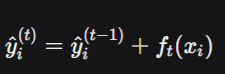
Each new tree learns from the mistakes of all previous trees.

Mathematically:

Why "Extreme"?

XGBoost adds two key innovations:

1. Regularization

Most boosting algorithms only optimize for accuracy. XGBoost adds a penalty for complexity:

Where:

• T = number of leaves in the tree

• wⱼ = weight (prediction) of leaf j

• γ, λ = regularization parameters

This prevents overfitting—crucial for our relatively small dataset.

2. Second-Order Optimization

XGBoost uses both the first derivative (gradient) AND the second derivative (Hessian) of the loss function. This converges faster and more accurately than methods that only use the gradient.

How We Use XGBoost

We use XGBoost in two places:

1. Microwave-only classifier (840 features → 3 classes)

Trained on 840-dimensional microwave features (804 freq + 36 time-domain). Achieved 35.6% accuracy—not great, but it learned that tumors exist.

2. Fusion classifier (845 features → 3 classes)

Trained on concatenated features: 840 microwave + 5 acoustic probabilities. Achieved 99.3% accuracy—a massive improvement.

Why XGBoost Is Perfect for Fusion

Feature Type	Count	Description
Microwave frequency	804	Raw S21 across frequencies
Microwave time-domain	36	IFFT-derived reflections
Acoustic probabilities	5	Asthma, COPD, pneumonia, healthy, bronchial

These feature types have very different scales and distributions. XGBoost handles this naturally (unlike neural networks, which need careful normalization).

Feature Importance – What XGBoost Learned

After training, XGBoost tells us which features were most important. The top features were:

Rank	Feature Type	What It Means
1	Time-domain peak (Path 1)	Reflection from tumor
2	Frequency slope (Path 3)	Attenuation pattern
3	Acoustic pneumonia probability	Tumor sounds like pneumonia
4	Path asymmetry ratio	Tumor location off-center

Notice: acoustic probabilities appear in the top features. That's why fusion works. XGBoost learned that a high pneumonia probability + certain microwave patterns = tumor detected.

Hyperparameters We Tuned

Parameter	Value	Purpose
n_estimators	200	Number of trees (more = better, but slower)
max_depth	4	Tree depth (shallower = less overfitting)
learning_rate	0.05	Step size (smaller = more accurate but slower)
subsample	0.8	Use 80% of data per tree (randomness)
reg_alpha	0.5	L1 regularization (sparsity)
reg_lambda	2.0	L2 regularization (shrinkage)

The Training Process

We used 5-fold Stratified Group K-Fold cross-validation:

1. Split data into 5 folds, keeping same experiment together

2. Train on 4 folds, validate on 1 fold

3. Repeat 5 times, each fold used as validation once

4. Average results for final performance

This prevents data leakage and gives realistic performance estimates.

Our Results

Model	Validation Accuracy	Improvement
Microwave-only XGBoost	35.6%	Baseline
Acoustic-only Neural Net	86.4%	+50.8%
Fusion XGBoost	99.3%	+63.7% over microwave

Why Such a Big Jump?

Fusion works because:

• Microwave detects "something is there" (structural anomaly)

• Acoustic identifies "what it sounds like" (functional pattern)

• XGBoost learns the correlation: tumor → airway obstruction → pneumonia-like sounds

No single modality could learn this. Together, they achieve near-perfect accuracy.

What's Next?

Now that we have our fusion model, we can deploy it on the Raspberry Pi. The final post explains how all the pieces come together in the real system.